pytorch0.4支持了Windows系统的开发,在首页即可使用pip安装pytorch和torchvision。
说白了,以下文字就是来自官方文档60分钟入门的简要翻译.
pytorch是啥
python的科学计算库,使得NumPy可用于GPU计算,并提供了一个深度学习平台使得灵活性和速度最大化
入门
Tensors(张量)
Tensors与NumPy的ndarrays类似,另外可以使用GPU加速计算
未初始化的5*3的矩阵:x = torch.empty(5, 3)
随机初始化的矩阵:x = torch.rand(5, 3)
全零矩阵,定义数据类型:x = torch.zeros(5, 3, dtype=torch.long)
由数据构造矩阵:x = torch.tensor([5.5, 3])
由已存在张量构造矩阵,性质与之前张量一致:1
2x = x.new_ones(5, 3, dtype=torch.double)
x = torch.randn_like(x, dtype=torch.float)
获取维度:print(x.size())
Operations
有多种operation的格式,这里考虑加法
1.
1 | y = torch.rand(5, 3) |
2.
1 | print(torch.add(x, y)) |
3.
1 | result = torch.empty(5, 3) |
4.
1 | # adds x to y |
operations中需要改变张量本身的值,可以在operation后加,比如`x.copy(y), x.t_()`
索引:print(x[:, 1])
改变维度:x.view(-1, 8)
和Numpy的联系
torch tensor 和 numpy array之间可以进行相互转换,他们会共享内存位置,改变一个,另一个会跟着改变。
tensor to array
1 | a = torch.ones(5) |
array to tensor
1 | import numpy as np |
CUDA Tensors
tensor可以使用.to方法将其移动到任何设备。
1 | # let us run this cell only if CUDA is available |
Autograd(自动求导)
pytorch神经网络的核心模块就是autograd,autograd模块对Tensors上的所有operations提供了自动求导。
Tensor
torch.Tensor是模块中的核心类,如果设置属性.requires_grad = True,开始追踪张量上的所有节点操作,指定其是否计算梯度。使用.backward()方法进行所有梯度的自动求导,张量的梯度会累积到.grad属性中。.detach()停止张量的追踪,从梯度计算中分离出来;另外在评估模型时一般使用代码块with torch.no_grad():,因为模型中通常训练的参数也会有.requires_grad = True,这样写可以停止全部张量的梯度更新。Function类是autograd的变体,Tensor和Function相互交错构建成无环图,编码了完整的计算过程,每个Variable(变量)都有.grad_fn属性,引用一个已经创建了的Tensor的Function.
如上,使用.backward()计算梯度。如果张量是一个标量(只有一个元素),不需要对.backward()指定参数;如果张量不止一个元素,需要指定.backward()的参数,其匹配张量的维度。
1 | import torch |
Gradients
反向传播时,由于out是一个标量,out.backward()等效于out.backward(torch.tensor(1))
1 | out.backward() |
神经网络
神经网络可以用torch.nn构建。nn依赖于autograd定义模型和求导,nn.Module定义网络层,方法forward(input)返回网络输出。
举例说明,如下是对数字图片分类的卷积网络架构。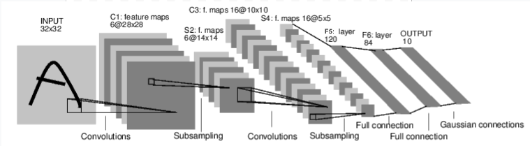
这是一个简单的前馈神经网络,将输入数据依次通过几层网络层后最终得到输出。
神经网络典型的训练步骤如下:
- 定义神经网络及学习的参数(权重)
- 迭代输入数据
- 将输入数据输入到网络结构中
- 计算代价函数
- 误差向后传播
- 更新网络权重
weight = weight - learning_rate * gradient
定义网络
1 | import torch |
out:1
2
3
4
5
6
7Net(
(conv1): Conv2d(1, 6, kernel_size=(5, 5), stride=(1, 1))
(conv2): Conv2d(6, 16, kernel_size=(5, 5), stride=(1, 1))
(fc1): Linear(in_features=400, out_features=120, bias=True)
(fc2): Linear(in_features=120, out_features=84, bias=True)
(fc3): Linear(in_features=84, out_features=10, bias=True)
)
可以仅定义forward()函数,当使用autograd时backward()被自动定义。可以在forward()函数中使用任何operation操作。net.parameters()返回模型中的可学习参数。
1 | params = list(net.parameters()) |
使所有参数的梯度归零然后开始计算梯度
1 | net.zero_grad() |
代价函数
代价函数将(output,target)作为输入,计算output与target之间的距离。
nn模块中有几种不同的代价函数选择,最简单的是nn.MSELoss,计算均方误差
eg:1
2
3
4
5
6
7output = net(input)
target = torch.arange(1, 11) # a dummy target, for example
target = target.view(1, -1) # make it the same shape as output
criterion = nn.MSELoss()
loss = criterion(output, target)
print(loss)
按照向后传播的方向传播loss,使用grad_fn可以查看整个流程的计算图1
2
3
4input -> conv2d -> relu -> maxpool2d -> conv2d -> relu -> maxpool2d
-> view -> linear -> relu -> linear -> relu -> linear
-> MSELoss
-> loss
使用loss.backward(),流程中所有requres_grad=True的张量累积它的梯度至.grad1
2
3print(loss.grad_fn) # MSELoss
print(loss.grad_fn.next_functions[0][0]) # Linear
print(loss.grad_fn.next_functions[0][0].next_functions[0][0]) # ReLU
向后传播
loss.backward()传播误差,1
2
3
4
5
6
7
8
9net.zero_grad() # zeroes the gradient buffers of all parameters
print('conv1.bias.grad before backward')
print(net.conv1.bias.grad)
loss.backward()
print('conv1.bias.grad after backward')
print(net.conv1.bias.grad)
更新权重
误差每次传播后,需要对权重进行更新,简单的更新方式如下:1
2
3learning_rate = 0.01
for f in net.parameters():
f.data.sub_(f.grad.data * learning_rate)
torch.optim实现了这一过程,并有着不同的更新规则GD, Nesterov-SGD, Adam, RMSProp,
1 | import torch.optim as optim |
note: 每次迭代时由于梯度的累积,需要手动将梯度归零optimizer.zero_grad()